Automatización
Álvaro Paredes y Carlos Lara
21 Julio de 2017
1 Los pendientes
¿Cómo les fue con la tarea?
set.seed(123)  # Para obtener el mismo resultado siempre... ¿aleatoriedad real?
ndays <- 52    # "Ciclos" por año
data_b <- rep(cos(seq(0, 2*pi, length.out=ndays)), 6) # 6 "años" de datos
data_base <- ((data_b + 1) * 5 + 10)  # Estacionalidad
ruido1 <- runif(length(data_base), -10, 10)  # Ruido
tendencia <- seq(0, 3, length.out = length(data_b)) # Tendencia
serie <- as.numeric(data_base + ma(ruido1, order=3) + tendencia) # Pillería: ma
serie[is.na(serie)] <- (data_base + tendencia)[is.na(serie)] # Reemplazo NAs
tiempo <- as.Date(paste0(rep(1:ndays*7), "-", rep(2000:2005, each=ndays)), "%j-%Y")
fin <- data.frame(fecha=tiempo, temperatura=serie, stringsAsFactors=F)
plot(temperatura~fecha, data=fin, type="l")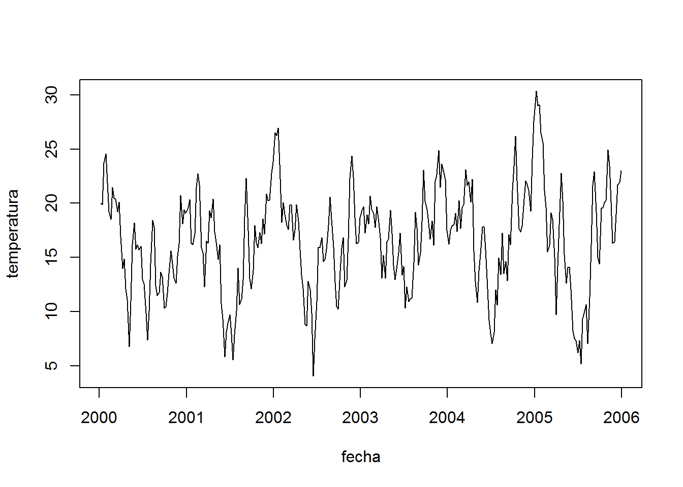
1.2 Gráfico con colores
var <- "month"
f_var <- as.numeric(as.factor(df[, var]))
nvar <- length(unique(df[, var]))
par(mar=c(5.1, 4.1, 4.1, 8.1), xpd=TRUE, bg="grey70")
plot(df$date, df$EVI, type="p", xlab="Year", ylab="EVI",
     main=paste0("The third best plot?: ", var),
     bty="n", xaxt="n", yaxt="n",
     col=topo.colors(nvar)[f_var],
     family="mono", pch=16, cex=.8)
axis(2, las=2, cex.axis=.8)
axis(1, las=1, cex.axis=.8,
     at=df$date[0:(length(unique(df$year)) - 1) * 12 + 1],
     labels=sort(unique(df$year)))
legend("bottomright",
       legend=sort(unique(df[, var])),
       col=topo.colors(nvar)[sort(unique(f_var))], pch=16, inset=c(-0.2,0))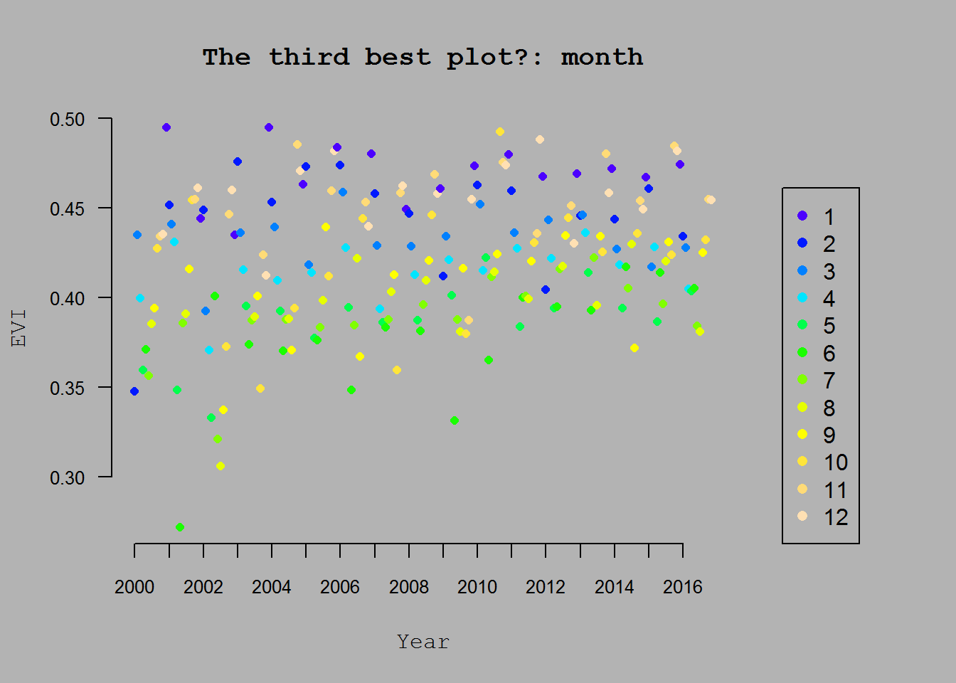
par(bg="white", mar=c(5.1,4.1,4.1,2.1))1.3 Gráfico con 2 ejes Y
set.seed(4598)
fake1 <- data.frame(x=1:20, Tp=sort(rnorm(20, 30, 4)), H=runif(20)*10+10)
# Modificar márgenes INTERNOS para dar más espacio izquierda y derecha
par(mar = c(5.1,5.1,4.1,5.1))   # márgenes abajo, izquierda, arriba, derecha
with(fake1, plot(x, Tp, type="l", col="black",
                 ylab=expression((sqrt(Tp))^2),
                 ylim=c(min(fake1), max(fake1)),
                 main="Gráfico Falso Falso"))
par(new=T)
with(fake1, plot(x, H, type="l", axes=F, xlab=NA, ylab=NA, col="darkgreen", lty=2))
axis(side = 4, col="darkgreen", col.axis="darkgreen")
mtext(side = 4, line = 3, 'Personas', col="darkgreen")
legend("bottomright",
       legend=c(expression((sqrt(Tp))^2), "Personas"),
       text.col=c("black", "darkgreen"),
       lty=c(1,2), col=c("black", "darkgreen"))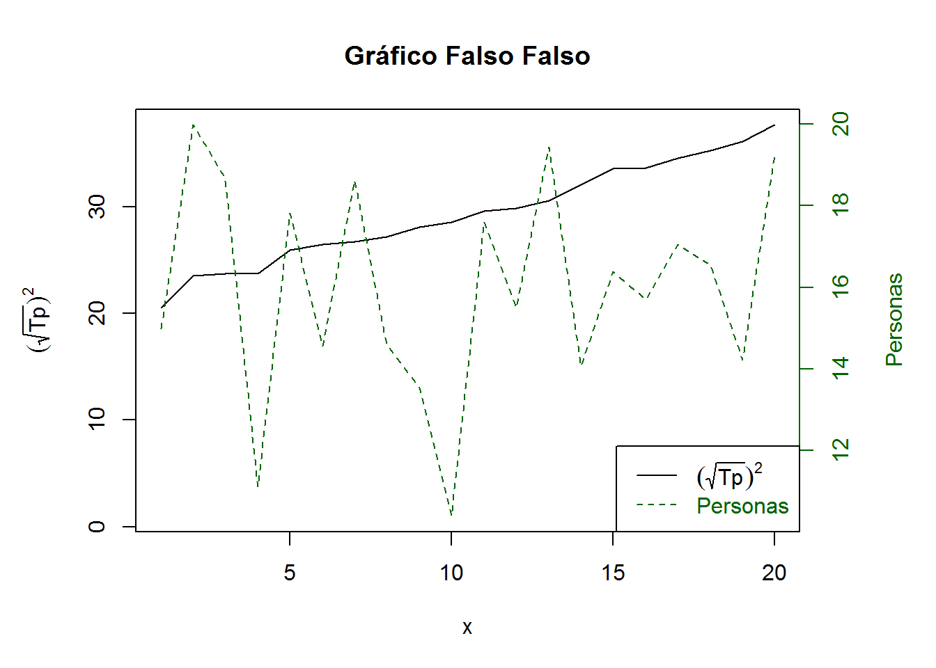
par(bg="white", mar=c(5,4,4,2)+.1) # Configuración original1.4 Gráfico con más de 3 ejes Y
Por si acaso….
set.seed(4598)
fake1 <- data.frame(x=1:20, Tp=sort(rnorm(20, 30, 4)), H=runif(20)*10+10, M=rnorm(10, 15, 1))
par(mar = c(5,8,4,4)+.1)   # márgenes abajo, izquierda, arriba, derecha
with(fake1, plot(x, Tp, type="l", col="black", axes=F, lwd=2,
                 ylim=c(min(fake1), max(fake1)), ylab=NA, xlab=NA,
                 main="Gráfico Falso Falso"))
axis(2, col="black", lwd=2)
mtext(2, line=2, col="black", text=c(expression((sqrt(Tp))^2)))

par(new=T)
with(fake1, plot(x, H, type="l", axes=F, xlab=NA, ylab=NA, col="darkgreen", lty=2))
axis(side = 4, col="darkgreen", col.axis="darkgreen")
mtext(side = 4, line = 2, 'Personas', col="darkgreen")

par(new=T)
with(fake1, plot(x, M, type="l", axes=F, xlab=NA, ylab=NA, col="blue3", lty=3))
axis(side = 2, line = 4.5, col="blue3", col.axis="blue3")
mtext(side = 2, line = 7, 'Nº Mariposas', col="blue3")

axis(1, at=pretty(0:20))
mtext("Tiempo temporal", side=1, line=2, col="black")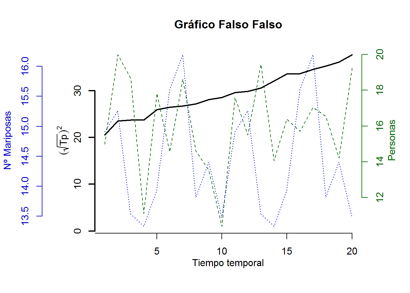
par(bg="white", mar=c(5,4,4,2)+.1) # Configuración original2 Otros análisis
2.1 Correlaciones
Tipos de correlaciones:
- Pearson
- Spearman
- Kendall
head(state.x77)## Population Income Illiteracy Life Exp Murder HS Grad Frost
## Alabama 3615 3624 2.1 69.05 15.1 41.3 20
## Alaska 365 6315 1.5 69.31 11.3 66.7 152
## Arizona 2212 4530 1.8 70.55 7.8 58.1 15
## Arkansas 2110 3378 1.9 70.66 10.1 39.9 65
## California 21198 5114 1.1 71.71 10.3 62.6 20
## Colorado 2541 4884 0.7 72.06 6.8 63.9 166
## Area
## Alabama 50708
## Alaska 566432
## Arizona 113417
## Arkansas 51945
## California 156361
## Colorado 103766cov(state.x77)## Population Income Illiteracy Life Exp
## Population 19931683.7588 571229.7796 292.8679592 -407.8424612
## Income 571229.7796 377573.3061 -163.7020408 280.6631837
## Illiteracy 292.8680 -163.7020 0.3715306 -0.4815122
## Life Exp -407.8425 280.6632 -0.4815122 1.8020204
## Murder 5663.5237 -521.8943 1.5817755 -3.8694804
## HS Grad -3551.5096 3076.7690 -3.2354694 6.3126849
## Frost -77081.9727 7227.6041 -21.2900000 18.2867796
## Area 8587916.9494 19049013.7510 4018.3371429 -12294.1022122
## Murder HS Grad Frost Area
## Population 5663.523714 -3551.509551 -77081.97265 8587916.949
## Income -521.894286 3076.768980 7227.60408 19049013.751
## Illiteracy 1.581776 -3.235469 -21.29000 4018.337
## Life Exp -3.869480 6.312685 18.28678 -12294.102
## Murder 13.627465 -14.549616 -103.40600 71940.430
## HS Grad -14.549616 65.237894 153.99216 229873.193
## Frost -103.406000 153.992163 2702.00857 262703.893
## Area 71940.429959 229873.192816 262703.89306 7280748060.842cor(state.x77)## Population Income Illiteracy Life Exp Murder
## Population 1.00000000 0.2082276 0.10762237 -0.06805195 0.3436428
## Income 0.20822756 1.0000000 -0.43707519 0.34025534 -0.2300776
## Illiteracy 0.10762237 -0.4370752 1.00000000 -0.58847793 0.7029752
## Life Exp -0.06805195 0.3402553 -0.58847793 1.00000000 -0.7808458
## Murder 0.34364275 -0.2300776 0.70297520 -0.78084575 1.0000000
## HS Grad -0.09848975 0.6199323 -0.65718861 0.58221620 -0.4879710
## Frost -0.33215245 0.2262822 -0.67194697 0.26206801 -0.5388834
## Area 0.02254384 0.3633154 0.07726113 -0.10733194 0.2283902
## HS Grad Frost Area
## Population -0.09848975 -0.3321525 0.02254384
## Income 0.61993232 0.2262822 0.36331544
## Illiteracy -0.65718861 -0.6719470 0.07726113
## Life Exp 0.58221620 0.2620680 -0.10733194
## Murder -0.48797102 -0.5388834 0.22839021
## HS Grad 1.00000000 0.3667797 0.33354187
## Frost 0.36677970 1.0000000 0.05922910
## Area 0.33354187 0.0592291 1.00000000cor(state.x77, method="spearman")## Population Income Illiteracy Life Exp Murder
## Population 1.0000000 0.12460984 0.3130496 -0.1040171 0.3457401
## Income 0.1246098 1.00000000 -0.3145948 0.3241050 -0.2174623
## Illiteracy 0.3130496 -0.31459482 1.0000000 -0.5553735 0.6723592
## Life Exp -0.1040171 0.32410498 -0.5553735 1.0000000 -0.7802406
## Murder 0.3457401 -0.21746230 0.6723592 -0.7802406 1.0000000
## HS Grad -0.3833649 0.51048095 -0.6545396 0.5239410 -0.4367330
## Frost -0.4588526 0.19686382 -0.6831936 0.2983910 -0.5438432
## Area -0.1206723 0.05709484 -0.2503721 0.1275002 0.1064259
## HS Grad Frost Area
## Population -0.3833649 -0.4588526 -0.12067227
## Income 0.5104809 0.1968638 0.05709484
## Illiteracy -0.6545396 -0.6831936 -0.25037208
## Life Exp 0.5239410 0.2983910 0.12750018
## Murder -0.4367330 -0.5438432 0.10642590
## HS Grad 1.0000000 0.3985351 0.43897520
## Frost 0.3985351 1.0000000 0.11228778
## Area 0.4389752 0.1122878 1.00000000Viendo la significancia:
state <- as.data.frame(state.x77)
with(state, cor.test(Population, Illiteracy))
##
## Pearson's product-moment correlation
##
## data: Population and Illiteracy
## t = 0.74999, df = 48, p-value = 0.4569
## alternative hypothesis: true correlation is not equal to 0
## 95 percent confidence interval:
## -0.1759976 0.3747441
## sample estimates:
## cor
## 0.10762242.2 T-tests
Para casos independientes:
library(MASS)
head(UScrime)
## M So Ed Po1 Po2 LF M.F Pop NW U1 U2 GDP Ineq Prob Time
## 1 151 1 91 58 56 510 950 33 301 108 41 394 261 0.084602 26.2011
## 2 143 0 113 103 95 583 1012 13 102 96 36 557 194 0.029599 25.2999
## 3 142 1 89 45 44 533 969 18 219 94 33 318 250 0.083401 24.3006
## 4 136 0 121 149 141 577 994 157 80 102 39 673 167 0.015801 29.9012
## 5 141 0 121 109 101 591 985 18 30 91 20 578 174 0.041399 21.2998
## 6 121 0 110 118 115 547 964 25 44 84 29 689 126 0.034201 20.9995
## y
## 1 791
## 2 1635
## 3 578
## 4 1969
## 5 1234
## 6 682t.test(Prob ~ So, data=UScrime)##
## Welch Two Sample t-test
##
## data: Prob by So
## t = -3.8954, df = 24.925, p-value = 0.0006506
## alternative hypothesis: true difference in means is not equal to 0
## 95 percent confidence interval:
## -0.03852569 -0.01187439
## sample estimates:
## mean in group 0 mean in group 1
## 0.03851265 0.06371269Los Estados (So) tienen diferentes probabilidades de encarcelamiento (Se rechaza la hipótesis de que tienen igual probabilidad).
Para casos dependientes:
sapply(UScrime[c("U1", "U2")], function(x)(c(mean=mean(x), sd=sd(x))))## U1 U2
## mean 95.46809 33.97872
## sd 18.02878 8.44545with(UScrime, t.test(U1, U2, paired=TRUE))##
## Paired t-test
##
## data: U1 and U2
## t = 32.407, df = 46, p-value < 0.00000000000000022
## alternative hypothesis: true difference in means is not equal to 0
## 95 percent confidence interval:
## 57.67003 65.30870
## sample estimates:
## mean of the differences
## 61.48936La diferencia entre las medias es bastante grande y la probabilidad muy pequeña; se rechaza la hipótesis de que el desempleo de hombres adultos es el mismo que el de los jóvenes (Adultos tienen mayor desempleo).
2.2.1 No paramétrico:
Si son independientes
with(UScrime, by(Prob, So, mean))## So: 0
## [1] 0.03851265
## --------------------------------------------------------
## So: 1
## [1] 0.06371269with(UScrime, by(Prob, So, median))## So: 0
## [1] 0.038201
## --------------------------------------------------------
## So: 1
## [1] 0.055552wilcox.test(Prob ~ So, data=UScrime)##
## Wilcoxon rank sum test
##
## data: Prob by So
## W = 81, p-value = 0.00008488
## alternative hypothesis: true location shift is not equal to 0O conocido también como “Mann–Whitney U test”; se rechaza la hipótesis de que ambos estados tienen las mismas probabilidades de encarcelamiento.
2.3 Modelos lineales
2.3.1 Simples
fit <- lm(dist ~ speed, data=cars)
fit
##
## Call:
## lm(formula = dist ~ speed, data = cars)
##
## Coefficients:
## (Intercept) speed
## -17.579 3.932summary(fit)##
## Call:
## lm(formula = dist ~ speed, data = cars)
##
## Residuals:
## Min 1Q Median 3Q Max
## -29.069 -9.525 -2.272 9.215 43.201
##
## Coefficients:
## Estimate Std. Error t value Pr(>|t|)
## (Intercept) -17.5791 6.7584 -2.601 0.0123 *
## speed 3.9324 0.4155 9.464 0.00000000000149 ***
## ---
## Signif. codes: 0 '***' 0.001 '**' 0.01 '*' 0.05 '.' 0.1 ' ' 1
##
## Residual standard error: 15.38 on 48 degrees of freedom
## Multiple R-squared: 0.6511, Adjusted R-squared: 0.6438
## F-statistic: 89.57 on 1 and 48 DF, p-value: 0.00000000000149names(fit)## [1] "coefficients" "residuals" "effects" "rank"
## [5] "fitted.values" "assign" "qr" "df.residual"
## [9] "xlevels" "call" "terms" "model"fitted(fit)## 1 2 3 4 5 6 7
## -1.849460 -1.849460 9.947766 9.947766 13.880175 17.812584 21.744993
## 8 9 10 11 12 13 14
## 21.744993 21.744993 25.677401 25.677401 29.609810 29.609810 29.609810
## 15 16 17 18 19 20 21
## 29.609810 33.542219 33.542219 33.542219 33.542219 37.474628 37.474628
## 22 23 24 25 26 27 28
## 37.474628 37.474628 41.407036 41.407036 41.407036 45.339445 45.339445
## 29 30 31 32 33 34 35
## 49.271854 49.271854 49.271854 53.204263 53.204263 53.204263 53.204263
## 36 37 38 39 40 41 42
## 57.136672 57.136672 57.136672 61.069080 61.069080 61.069080 61.069080
## 43 44 45 46 47 48 49
## 61.069080 68.933898 72.866307 76.798715 76.798715 76.798715 76.798715
## 50
## 80.731124residuals(fit)## 1 2 3 4 5 6
## 3.849460 11.849460 -5.947766 12.052234 2.119825 -7.812584
## 7 8 9 10 11 12
## -3.744993 4.255007 12.255007 -8.677401 2.322599 -15.609810
## 13 14 15 16 17 18
## -9.609810 -5.609810 -1.609810 -7.542219 0.457781 0.457781
## 19 20 21 22 23 24
## 12.457781 -11.474628 -1.474628 22.525372 42.525372 -21.407036
## 25 26 27 28 29 30
## -15.407036 12.592964 -13.339445 -5.339445 -17.271854 -9.271854
## 31 32 33 34 35 36
## 0.728146 -11.204263 2.795737 22.795737 30.795737 -21.136672
## 37 38 39 40 41 42
## -11.136672 10.863328 -29.069080 -13.069080 -9.069080 -5.069080
## 43 44 45 46 47 48
## 2.930920 -2.933898 -18.866307 -6.798715 15.201285 16.201285
## 49 50
## 43.201285 4.268876plot(cars$speed, cars$dist)
abline(fit, col="red")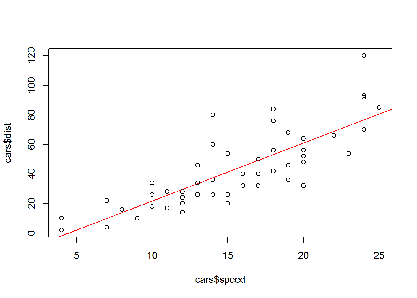
¿probemos con otro conjunto de datos?
2.3.2 Múltiple
library(car)
scatterplotMatrix(state, spread=FALSE, smoother.args=list(lty=2),
main="Scatter Plot Matrix")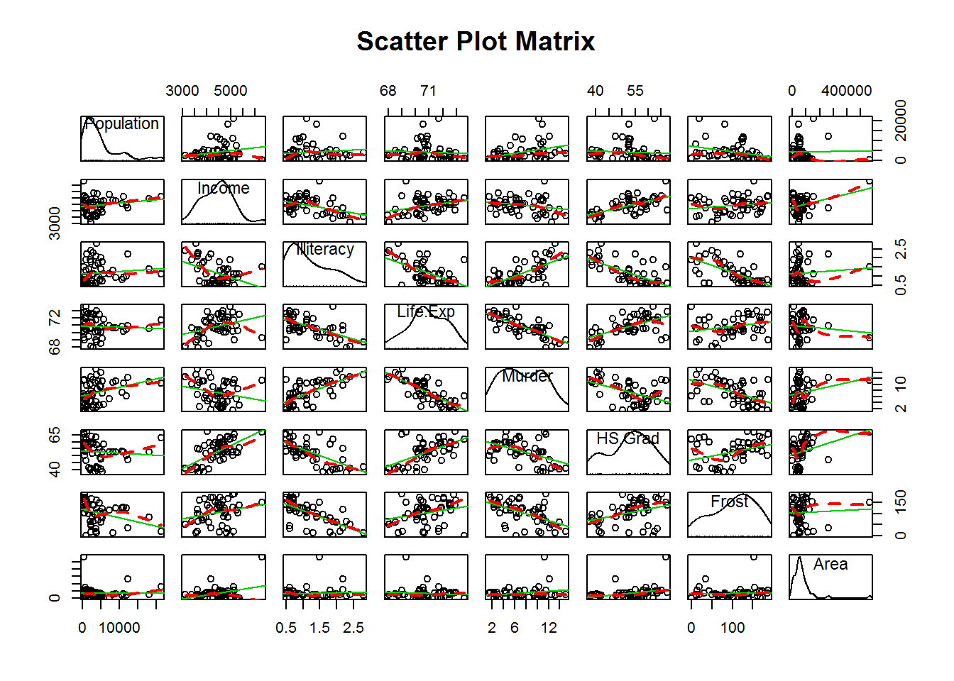
fit <- lm(Murder ~ Population + Illiteracy + Income + Area, data=state)
summary(fit)
##
## Call:
## lm(formula = Murder ~ Population + Illiteracy + Income + Area,
## data = state)
##
## Residuals:
## Min 1Q Median 3Q Max
## -3.9409 -1.7400 -0.2251 1.5436 7.5654
##
## Coefficients:
## Estimate Std. Error t value Pr(>|t|)
## (Intercept) 4.066402226 3.541037025 1.148 0.25689
## Population 0.000243274 0.000082316 2.955 0.00496 **
## Illiteracy 3.699008907 0.682156656 5.423 0.00000223 ***
## Income -0.000607782 0.000737242 -0.824 0.41406
## Area 0.000009143 0.000004591 1.992 0.05251 .
## ---
## Signif. codes: 0 '***' 0.001 '**' 0.01 '*' 0.05 '.' 0.1 ' ' 1
##
## Residual standard error: 2.43 on 45 degrees of freedom
## Multiple R-squared: 0.602, Adjusted R-squared: 0.5666
## F-statistic: 17.02 on 4 and 45 DF, p-value: 0.00000001446confint(fit)## 2.5 % 97.5 %
## (Intercept) -3.0656124457867 11.19841689777
## Population 0.0000774815040 0.00040906742
## Illiteracy 2.3250748745565 5.07294294019
## Income -0.0020926633692 0.00087709989
## Area -0.0000001034339 0.00001838864par(mfrow=c(2,2))
plot(fit)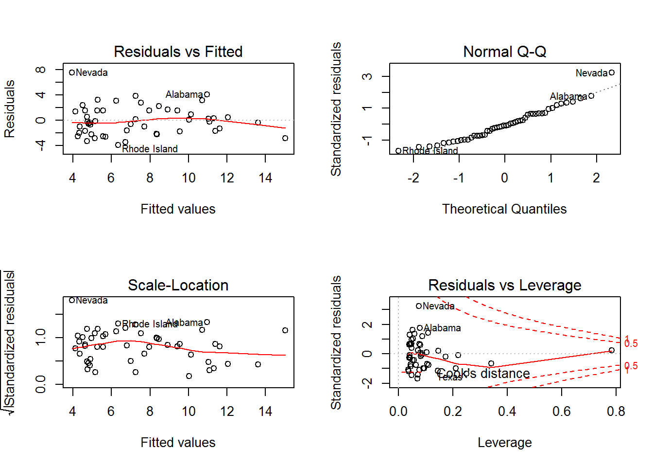
par(mfrow=c(1,1))2.3.3 Múltiple con interacciones
fit2 <- lm(mpg ~ hp + wt + hp:wt, data=mtcars)
summary(fit2)
##
## Call:
## lm(formula = mpg ~ hp + wt + hp:wt, data = mtcars)
##
## Residuals:
## Min 1Q Median 3Q Max
## -3.0632 -1.6491 -0.7362 1.4211 4.5513
##
## Coefficients:
## Estimate Std. Error t value Pr(>|t|)
## (Intercept) 49.80842 3.60516 13.816 0.0000000000000501 ***
## hp -0.12010 0.02470 -4.863 0.0000403624302068 ***
## wt -8.21662 1.26971 -6.471 0.0000005199287280 ***
## hp:wt 0.02785 0.00742 3.753 0.000811 ***
## ---
## Signif. codes: 0 '***' 0.001 '**' 0.01 '*' 0.05 '.' 0.1 ' ' 1
##
## Residual standard error: 2.153 on 28 degrees of freedom
## Multiple R-squared: 0.8848, Adjusted R-squared: 0.8724
## F-statistic: 71.66 on 3 and 28 DF, p-value: 0.0000000000002981Sería: \(mpg = 49.80 - 0.12*hp - 8.22*wt + 0.03*hp*wt\)
2.3.4 Ejemplo aplicado
Un modelo líneal puede ser tan simple como el anterior o tan complejo como el siguiente ejemplo:
\[ HT = 1.3 + (b0 + b1 * HD + b2 * D1) * (ntrees/(1 + ntrees))^{(c0 + c1 * age + c2 * log(tph) + c3 * BA + c4 * D1 + c5 * Hd * sqrt(tph))}\]
2.4 Normalidad
shapiro.test(rnorm(100, mean = 6, sd = 2))##
## Shapiro-Wilk normality test
##
## data: rnorm(100, mean = 6, sd = 2)
## W = 0.99331, p-value = 0.9062shapiro.test(runif(100, min = 1, max = 5))##
## Shapiro-Wilk normality test
##
## data: runif(100, min = 1, max = 5)
## W = 0.95353, p-value = 0.001428shapiro.test(df$EVI)##
## Shapiro-Wilk normality test
##
## data: df$EVI
## W = 0.98104, p-value = 0.007663EVI no es ¿normal?
2.5 ANOVA
Hay varioas formas de utilizar ANOVA y aquí veremos rápidamente algunas de ellas:
2.5.1 Una vía
library(multcomp)with(cholesterol, table(trt))## trt
## 1time 2times 4times drugD drugE
## 10 10 10 10 10aov1 <- aov(response ~ trt, data=cholesterol)
summary(aov1)## Df Sum Sq Mean Sq F value Pr(>F)
## trt 4 1351.4 337.8 32.43 0.000000000000982 ***
## Residuals 45 468.8 10.4
## ---
## Signif. codes: 0 '***' 0.001 '**' 0.01 '*' 0.05 '.' 0.1 ' ' 1TukeyHSD(aov1)## Tukey multiple comparisons of means
## 95% family-wise confidence level
##
## Fit: aov(formula = response ~ trt, data = cholesterol)
##
## $trt
## diff lwr upr p adj
## 2times-1time 3.44300 -0.6582817 7.544282 0.1380949
## 4times-1time 6.59281 2.4915283 10.694092 0.0003542
## drugD-1time 9.57920 5.4779183 13.680482 0.0000003
## drugE-1time 15.16555 11.0642683 19.266832 0.0000000
## 4times-2times 3.14981 -0.9514717 7.251092 0.2050382
## drugD-2times 6.13620 2.0349183 10.237482 0.0009611
## drugE-2times 11.72255 7.6212683 15.823832 0.0000000
## drugD-4times 2.98639 -1.1148917 7.087672 0.2512446
## drugE-4times 8.57274 4.4714583 12.674022 0.0000037
## drugE-drugD 5.58635 1.4850683 9.687632 0.0030633par(las=2, mar=c(5,8,4,2))
plot(TukeyHSD(aov1))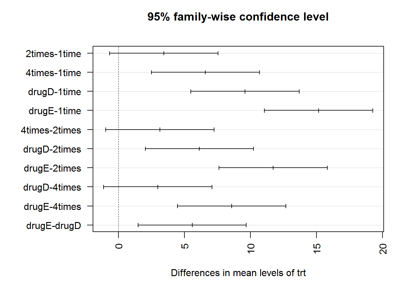
par(las=0, mar=c(5,4,4,2)+.1)

tuk <- glht(aov1, linfct=mcp(trt="Tukey"))
par(mar=c(5,4,6,2))
plot(cld(tuk, level=.05),col="gold")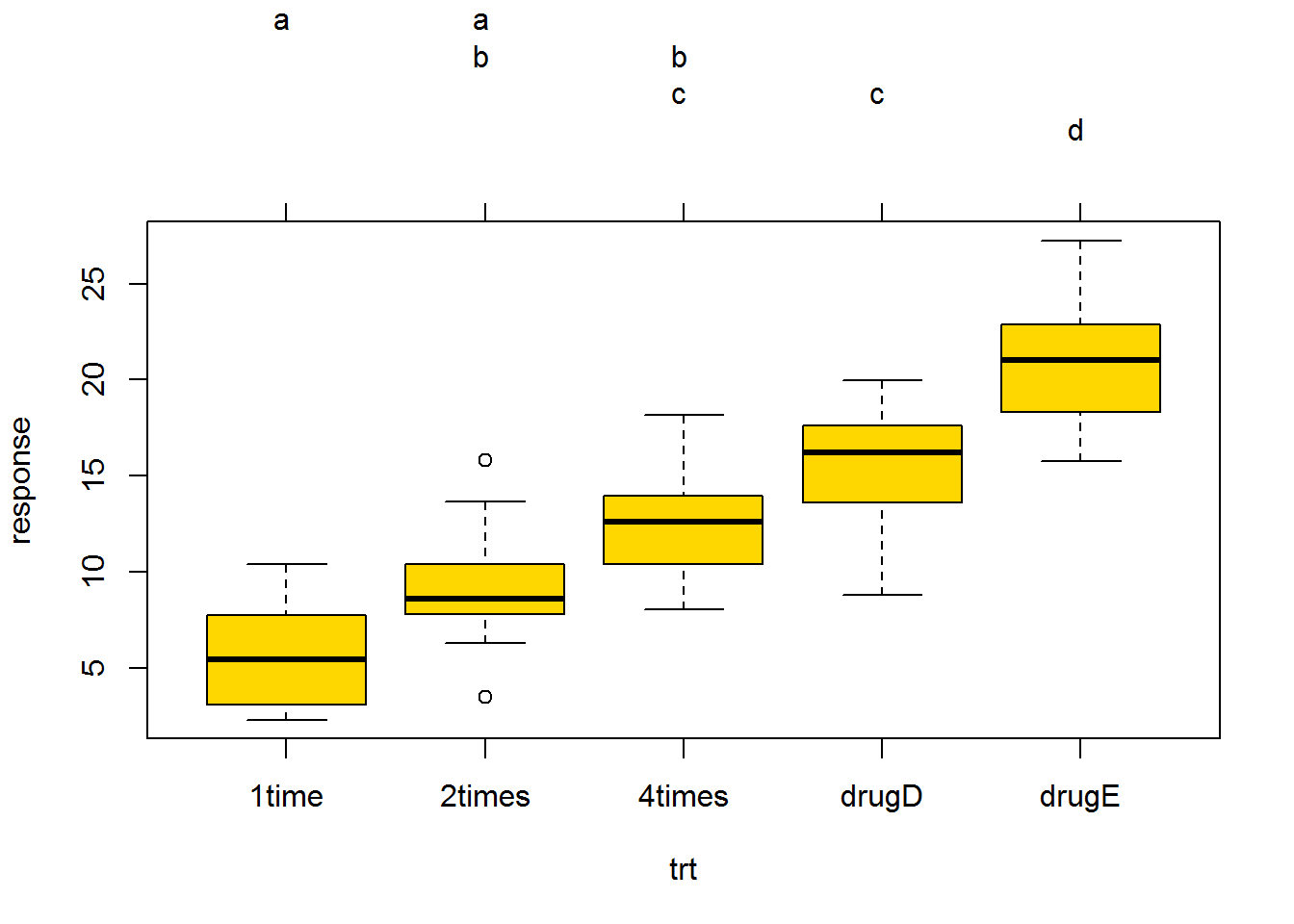
par(mar=c(5,4,4,2)+.1)2.5.2 Dos vías factorial
head(ToothGrowth)## len supp dose
## 1 4.2 VC 0.5
## 2 11.5 VC 0.5
## 3 7.3 VC 0.5
## 4 5.8 VC 0.5
## 5 6.4 VC 0.5
## 6 10.0 VC 0.5with(ToothGrowth, table(supp, dose))## dose
## supp 0.5 1 2
## OJ 10 10 10
## VC 10 10 10ToothGrowth$dose <- factor(ToothGrowth$dose)
aov2 <- aov(len ~ supp*dose, data=ToothGrowth)
summary(aov2)## Df Sum Sq Mean Sq F value Pr(>F)
## supp 1 205.4 205.4 15.572 0.000231 ***
## dose 2 2426.4 1213.2 92.000 < 2e-16 ***
## supp:dose 2 108.3 54.2 4.107 0.021860 *
## Residuals 54 712.1 13.2
## ---
## Signif. codes: 0 '***' 0.001 '**' 0.01 '*' 0.05 '.' 0.1 ' ' 13 Bucles
for (i in 1:10) {
  print(paste0("¡Soy el número ", i, "!"))
}
## [1] "¡Soy el número 1!"
## [1] "¡Soy el número 2!"
## [1] "¡Soy el número 3!"
## [1] "¡Soy el número 4!"
## [1] "¡Soy el número 5!"
## [1] "¡Soy el número 6!"
## [1] "¡Soy el número 7!"
## [1] "¡Soy el número 8!"
## [1] "¡Soy el número 9!"
## [1] "¡Soy el número 10!"A construir un bucle para probar varias combinaciones de ARIMA con los datos del índice EVI.
4 Funciones
soy_numero <- function(num) {


  if (any(num < 0)) stop("¡Sólo números positivos!")
  if (length(num) > 1) {
    it <- num
  } else {
    it <- 1:num
  }
  for (i in it) {
    print(paste0("¡Soy el número ", i, "!"))
  }
  return(it)
}

soy_numero(13)
## [1] "¡Soy el número 1!"
## [1] "¡Soy el número 2!"
## [1] "¡Soy el número 3!"
## [1] "¡Soy el número 4!"
## [1] "¡Soy el número 5!"
## [1] "¡Soy el número 6!"
## [1] "¡Soy el número 7!"
## [1] "¡Soy el número 8!"
## [1] "¡Soy el número 9!"
## [1] "¡Soy el número 10!"
## [1] "¡Soy el número 11!"
## [1] "¡Soy el número 12!"
## [1] "¡Soy el número 13!"## [1] 1 2 3 4 5 6 7 8 9 10 11 12 13soy_numero(c(1, 10:12))## [1] "¡Soy el número 1!"
## [1] "¡Soy el número 10!"
## [1] "¡Soy el número 11!"
## [1] "¡Soy el número 12!"## [1] 1 10 11 12Construyamos una función ahora, que automatice las combinaciones de ARIMA con cualquier serie de tiempo.
5 Extras
Una buena guía para comenzar con determinados análisis
Para comparar dos series de tiempo, el paquete TSdist puede ser de utilidad
Una guía con algunas de los símbolos para las formulaciones de los modelos líneales
Algunos ejemplos están basados en el libro “R in Action”: Correlaciones, T-Test, lm múltiple y ANOVA